OpenSees Basic Examples (H5: 弾性フレーム解析) コマンドサマリ

Basic Examples Manual (Elastic Frame Example)　解説
のコマンドのサマリは以下の通りです。

このコマンドを　ファイル名　ElasticFrame.tcl　として、テキストフォーマットで作成し、


OpenSeesの起動環境　で　起動しているOpenSees のコマンドラインに


OpenSees ElasticFrame.tcl  <Enter>

と打ち込んで、実行します。


----- ElasticFrame.tcl 始まり　------

# OpenSees -- Open System for Earthquake Engineering Simulation

# Pacific Earthquake Engineering Research Center

# http://opensees.berkeley.edu/

#

# Basic Elastic Frame

# ----------------------

#  2d Elastic Beam Column Elements

#  Distributed Load & Pushover Analysis

# 

# Example Objectives

# -----------------

#  Simple Introduction to OpenSees

# 

# Units: kips, in, sec

# Written: fmk

# Date: January 2011

#

# set some parameter

#

set PI  [expr 2.0 * asin(1.0)]

set g   386.4

set ft  12.0

set Load1 1185.0; 

set Load2 1185.0; 

set Load3  970.0;

# set floor masses 質量

set m1  [expr $Load1/(4*$g)]; # 4 nodes per floor

set m2  [expr $Load2/(4*$g)]

set m3  [expr $Load3/(4*$g)]

# set floor distributed loads

set w1  [expr $Load1/(90*$ft)];   # frame 90 ft long (1ft = 12in)

set w2  [expr $Load2/(90*$ft)]

set w3  [expr $Load3/(90*$ft)]

# ------------------------------

# Start of model generation

# ------------------------------

# Remove existing model

wipe

# Create ModelBuilder (with two-dimensions and 2 DOF/node)

model BasicBuilder -ndm 2 -ndf 3

# Create nodes

# ------------

# Create nodes & add to Domain - command: node nodeId xCrd yCrd <-mass $massX $massY $massRz>

# NOTE: mass in optional

node 1     0.0   0.0 

node 2   360.0   0.0 

node 3   720.0   0.0 

node 4  1080.0   0.0 

node 5    0.0  162.0 -mass $m1 $m1 0.0

node 6  360.0  162.0 -mass $m1 $m1 0.0

node 7  720.0  162.0 -mass $m1 $m1 0.0

node 8 1080.0  162.0 -mass $m1 $m1 0.0

node 9     0.0 324.0 -mass $m2 $m2 0.0

node 10  360.0 324.0 -mass $m2 $m2 0.0

node 11  720.0 324.0 -mass $m2 $m2 0.0

node 12 1080.0 324.0 -mass $m2 $m2 0.0

node 13    0.0 486.0 -mass $m3 $m3 0.0

node 14  360.0 486.0 -mass $m3 $m3 0.0

node 15  720.0 486.0 -mass $m3 $m3 0.0

node 16 1080.0 486.0 -mass $m3 $m3 0.0

# Set the boundary conditions - command: fix nodeID xResrnt? yRestrnt? rZRestrnt?

fix 1 1 1 1

fix 2 1 1 1

fix 3 1 1 1

fix 4 1 1 1

# Define geometric transformations for beam-column elements

geomTransf Linear 1; # beams

geomTransf PDelta 2; # columns

# Define elements

# Create elastic beam-column - command: element elasticBeamColumn eleID node1 node2 A E Iz geomTransfTag

# Define the Columns

#[ elementの番号 ] [ 片方のnode番号] [片方のnode番号] [ 断面積] [ヤング率] [Z軸の慣性モーメント] [$transfTag]

element elasticBeamColumn  1  1  5 75.6 29000.0 3400.0 2; # W14X257

element elasticBeamColumn  2  5  9 75.6 29000.0 3400.0 2; # W14X257

element elasticBeamColumn  3  9 13 75.6 29000.0 3400.0 2; # W14X257

element elasticBeamColumn  4  2  6 91.4 29000.0 4330.0 2; # W14X311

element elasticBeamColumn  5  6 10 91.4 29000.0 4330.0 2; # W14X311

element elasticBeamColumn  6 10 14 91.4 29000.0 4330.0 2; # W14X311

element elasticBeamColumn  7  3  7 91.4 29000.0 4330.0 2; # W14X311

element elasticBeamColumn  8  7 11 91.4 29000.0 4330.0 2; # W14X311

element elasticBeamColumn  9 11 15 91.4 29000.0 4330.0 2; # W14X311

element elasticBeamColumn 10  4  8 75.6 29000.0 3400.0 2; # W14X257

element elasticBeamColumn 11  8 12 75.6 29000.0 3400.0 2; # W14X257

element elasticBeamColumn 12 12 16 75.6 29000.0 3400.0 2; # W14X257

# Define the Beams

element elasticBeamColumn 13  5  6 34.7 29000.0 5900.0 1; # W33X118

element elasticBeamColumn 14  6  7 34.7 29000.0 5900.0 1; # W33X118

element elasticBeamColumn 15  7  8 34.7 29000.0 5900.0 1; # W33X118

element elasticBeamColumn 16  9 10 34.2 29000.0 4930.0 1; # W30X116

element elasticBeamColumn 17 10 11 34.2 29000.0 4930.0 1; # W30X116

element elasticBeamColumn 18 11 12 34.2 29000.0 4930.0 1; # W30X116

element elasticBeamColumn 19 13 14 20.1 29000.0 1830.0 1; # W24X68

element elasticBeamColumn 20 14 15 20.1 29000.0 1830.0 1; # W24X68

element elasticBeamColumn 21 15 16 20.1 29000.0 1830.0 1; # W24X68

# Define loads for Gravity Analysis

# ---------------------------------

#create a Linear TimeSeries (load factor varies linearly with time): command timeSeries Linear $tag

timeSeries Linear 1

# Create a Plain load pattern with a linear TimeSeries: 

#  command pattern Plain $tag $timeSeriesTag { $loads }

pattern Plain 1 1 {

    eleLoad -ele 13 14 15 -type -beamUniform -$w1

    eleLoad -ele 16 17 18 -type -beamUniform -$w2

    eleLoad -ele 19 20 21 -type -beamUniform -$w3

}

# ---------------------------------

# Create Analysis for Gravity Loads

# ---------------------------------

# Create the system of equation, a SPD using a band storage scheme

system BandSPD

# Create the DOF numberer, the reverse Cuthill-McKee algorithm

numberer RCM

# Create the constraint handler, a Plain handler is used as homo constraints

constraints Plain

# Create the integration scheme, the LoadControl scheme using steps of 1.0

integrator LoadControl 1.0

# Create the solution algorithm, a Linear algorithm is created

test NormDispIncr 1.0e-10 6

algorithm Newton

# create the analysis object 

analysis Static 

# ---------------------------------

# Perform Gravity Analysis

# ---------------------------------

analyze 1

# ---------------------------------

# Check Equilibrium

# ---------------------------------

# invoke command to determine nodal reactions 

reactions

set node1Rxn [nodeReaction 1]; # nodeReaction command returns nodal reactions for specified node in a list

set node2Rxn [nodeReaction 2]

set node3Rxn [nodeReaction 3]

set node4Rxn [nodeReaction 4]

set inputedFy  [expr -$Load1-$Load2-$Load3]; # loads added negative Fy diren to ele

set computedFx [expr [lindex $node1Rxn 0]+[lindex $node2Rxn 0]+[lindex $node3Rxn 0]+[lindex $node4Rxn 0]]

set computedFy [expr [lindex $node1Rxn 1]+[lindex $node2Rxn 1]+[lindex $node3Rxn 1]+[lindex $node4Rxn 1]]

puts "\nEqilibrium Check After Gravity:"

puts "SumX: Inputed: 0.0 + Computed: $computedFx = [expr 0.0+$computedFx]"

puts "SumY: Inputed: $inputedFy + Computed: $computedFy = [expr $inputedFy+$computedFy]"

# ---------------------------------

# Lateral Load

# ---------------------------------

# set gravity loads constant and time in domain to e 0.0

loadConst -time 0.0

timeSeries Linear 2

pattern Plain 2 2 {

    load 13 220.0 0.0 0.0

    load  9 180.0 0.0 0.0

    load  5  90.0 0.0 0.0

}

# ---------------------------------

# Create Recorder

# ---------------------------------

recorder Element -file EleForces.txt -ele 1 4 7 10 forces

# ---------------------------------

# Perform Lateral Analysis

# ---------------------------------

analyze 1

# ---------------------------------

# Check Equilibrium

# ---------------------------------

reactions

set node1Rxn [nodeReaction 1]; # nodeReaction command returns nodal reactions for specified node in a list

set node2Rxn [nodeReaction 2]

set node3Rxn [nodeReaction 3]

set node4Rxn [nodeReaction 4]

set inputedFx  [expr 220.0+180.0+90.0] 

set computedFx [expr [lindex $node1Rxn 0]+[lindex $node2Rxn 0]+[lindex $node3Rxn 0]+[lindex $node4Rxn 0]]

set computedFy [expr [lindex $node1Rxn 1]+[lindex $node2Rxn 1]+[lindex $node3Rxn 1]+[lindex $node4Rxn 1]]

puts "\nEqilibrium Check After Lateral Loads:"

puts "SumX: Inputed: $inputedFx + Computed: $computedFx = [expr $inputedFx+$computedFx]"

puts "SumY: Inputed: $inputedFy + Computed: $computedFy = [expr $inputedFy+$computedFy]"

# print ele information for columns at base

print ele 1 4 7 10

# ---------------------------------

# Check Eigenvalues

# ---------------------------------

set eigenValues [eigen 5]

puts "\nEigenvalues:"

set eigenValue [lindex $eigenValues 0]

puts "T[expr 0+1] = [expr 2*$PI/sqrt($eigenValue)]"

set eigenValue [lindex $eigenValues 1]

puts "T[expr 1+1] = [expr 2*$PI/sqrt($eigenValue)]"

set eigenValue [lindex $eigenValues 2]

puts "T[expr 2+1] = [expr 2*$PI/sqrt($eigenValue)]"

set eigenValue [lindex $eigenValues 3]

puts "T[expr 3+1] = [expr 2*$PI/sqrt($eigenValue)]"

set eigenValue [lindex $eigenValues 4]

puts "T[expr 4+1] = [expr 2*$PI/sqrt($eigenValue)]"

recorder Node -file eigenvector.txt -nodeRange 5 16 -dof 1 2 3 eigen 0

record

exit

----- ElasticFrame.tcl  終わり　------

次のページ　→
Basic Examples Manual (Elastic Frame Example)　
解析結果

Opensees コマンド　日本語解説　： 目次

OpenSees Basic Examples H4: (弾性フレーム解析) 解説 (Lateral Load 横荷重)

6）横荷重の設定

この構造物に加える重力荷重（オレンジの矢印部分）を設定します。

解析する時間をリセットします
loadConst -time [リセットする値]  
ｌoadConst -time 0.0

timeSeries Linear [タグ番号]　
このコマンドについての説明は、ここ。
「時間ごとに線形に一様に変位する力」という定義です。

pattern Plain [Loadの通し番号] [ 上記のtimeSeriesで指定したタグ番号]  {
     load [Node番号] [自由度の１番目に対してかける力（X方向)] [ 自由度の１番目に対してかける力（Y方向)] 
      [ 自由度の3番目に対してかける力（θ方向)]
}

timeSeries Linear 2
pattern Plain 2 2 {
    load 13 220.0 0.0 0.0
    load  9 180.0 0.0 0.0
    load  5  90.0 0.0 0.0
}

7）レコーダーの設定

ここでは、Recorder Element コマンド　を使用します

recorder Element -file EleForces.txt -ele 1 4 7 10 forces

（参照ページはここ）

8）解析開始
ここでは、解析を１行のみ行うように指定しています。
（参照ページは、ここ）

analyze 1

9) 平衡点(バランス）のチェックと結果表示

「analyze 1 」の結果は、もしRecorderコマンドでの出力ファイルの指定があった場合は、このファイルに結果を出力します。（参照ページは　ここ）

ここではスクリーン上に出力します。

抗力の結果を出力することを指示するコマンド
# invoke command to determine nodal reactions 
reactions

Node1,2,3,4の抗力を、node1Rxn, node2Rxn, node3Rxn, node4Rxn にセットします
# nodeReaction command returns nodal reactions for specified node in a list
set node1Rxn [nodeReaction 1]; 
set node2Rxn [nodeReaction 2]
set node3Rxn [nodeReaction 3]
set node4Rxn [nodeReaction 4]

Ｙ方向の想定される力は重力のみ　inputedFyには、ここで定義した固定荷重がセットされています。
X方向の想定される力として　inputedFxに、ここで定義した横荷重がセットされています。
set inputedFx  [expr 220.0+180.0+90.0] 




解析結果で出力されるＸ方向の抗力をcomputedFxにセットします
set computedFx [expr [lindex $node1Rxn 0]+[lindex $node2Rxn 0]+[lindex $node3Rxn 0]+[lindex $node4Rxn 0]]

解析結果で出力されるY方向の抗力をcomputedFyにセットします
set computedFy [expr [lindex $node1Rxn 1]+[lindex $node2Rxn 1]+[lindex $node3Rxn 1]+[lindex $node4Rxn 1]]

バランスチェックは、想定されていた力と、解析した力の残差で行います
puts "\nEqilibrium Check After Lateral Loads:"

X方向は、想定される力０と、computedFxの残差を計算します
puts "SumX: Inputed: $inputedFx + Computed: $computedFx = [expr $inputedFx+$computedFx]"
Ｙ方向は、inputedFyと、computedFyの残差を計算します
puts "SumY: Inputed: $inputedFy + Computed: $computedFy = [expr $inputedFy+$computedFy]"

Element(要素）1, 4, 7, 10の値を表示します

# print ele information for columns at base
print ele 1 4 7 10


10) 固有周期の表示

1次から５次までの固有周期を表示します
n次の固有値は、Eigen コマンド　で定義されています。
[eigen n]
eigenValueに1次から５次までの固有値をセットします。

set eigenValues [eigen 5]

puts "\nEigenvalues:"

λ：固有値　ω：固有振動数　T: 固有周期

１次の固有値から、固有周期をもとめます
set eigenValue [lindex $eigenValues 0]

puts "T[expr 0+1] = [expr 2*$PI/sqrt($eigenValue)]"

putコマンドにより　T[1] = に、１次固有周期　が表示されます。

同じように、
2次から５次までの固有値から、固有周期を求め、表示します。
set eigenValue [lindex $eigenValues 1]
puts "T[expr 1+1] = [expr 2*$PI/sqrt($eigenValue)]"
set eigenValue [lindex $eigenValues 2]
puts "T[expr 2+1] = [expr 2*$PI/sqrt($eigenValue)]"
set eigenValue [lindex $eigenValues 3]
puts "T[expr 3+1] = [expr 2*$PI/sqrt($eigenValue)]"
set eigenValue [lindex $eigenValues 4]
puts "T[expr 4+1] = [expr 2*$PI/sqrt($eigenValue)]"

次に、Recorder Node コマンドを使用して、

Node 5から16までの　３つの自由度の値を、１次固有振動モードから５次固有振動モードまで出力します。
（先に”eigen 5”とセットしたので、５次まで出力します）

recorder Node -file eigenvector.txt -nodeRange 5 16 -dof 1 2 3 eigen 0

現在もとめられている上記のデータを、ファイルに記録します
record

exit


次のページ　→

Basic Examples  (Elastic Frame)　
解説(コマンドのサマリ）

Opensees コマンド　日本語解説　： 目次

OpenSees Basic Examples (H3: 弾性フレーム解析) 解説(Gravity Loads 重力荷重)

2）重力荷重の設定

この構造物に加える重力荷重（紫の矢印部分）を設定します。

timeSeries Linear [タグ番号]　
このコマンドについての説明は、ここ。
「時間ごとに線形に一様に変位する力」という定義です。


また、Element(要素）にかける外力なので、Elemental Loadを使用します。
（参照ページはここ）
このコマンドは、一本線であらわされる要素に適用できるもので、連続体での要素には適用できません。

pattern Plain [Loadの通し番号] [ 上記のtimeSeriesで指定したタグ番号]  {
     eleLoad -ele [Element番号] -type -beamUniform [分散荷重]

timeSeries Linear 1

pattern Plain 1 1 {
    eleLoad -ele 13 14 15 -type -beamUniform -$w1
    eleLoad -ele 16 17 18 -type -beamUniform -$w2
    eleLoad -ele 19 20 21 -type -beamUniform -$w3
}



3）OpenSeesで用意されているツールの設定
有限要素法で使用する連立方程式の解法を設定します。
ここで使用しているコマンドについての
参照ページは　ここ　と　ここ


# Create the system of equation, a SPD using a band storage scheme
system BandSPD

# Create the DOF numberer, the reverse Cuthill-McKee algorithm
numberer RCM

# Create the constraint handler, a Plain handler is used as homo constraints
constraints Plain

# Create the integration scheme, the LoadControl scheme using steps of 1.0
integrator LoadControl 1.0

# Create the solution algorithm, a Linear algorithm is created
test NormDispIncr 1.0e-10 6
algorithm Newton

# create the analysis object 
analysis Static 

4）解析開始
ここでは、解析を１行のみ行うように指定しています。
（参照ページは、ここ）

analyze 1

5) 平衡点(バランス）のチェックと結果表示

「analyze 1 」の結果は、もしRecorderコマンドでの出力ファイルの指定があった場合は、このファイルに結果を出力します。（参照ページは　ここ）

ここではスクリーン上に出力します。

抗力の結果を出力することを指示するコマンド
# invoke command to determine nodal reactions 
reactions

Node1,2,3,4の抗力を、node1Rxn, node2Rxn, node3Rxn, node4Rxn にセットします
# nodeReaction command returns nodal reactions for specified node in a list
set node1Rxn [nodeReaction 1]; 
set node2Rxn [nodeReaction 2]
set node3Rxn [nodeReaction 3]
set node4Rxn [nodeReaction 4]

Ｙ方向の想定される力は重力のみ　inputedFyに、ここで定義した固定荷重をセットします。
# loads added negative Fy diren to ele
set inputedFy  [expr -$Load1-$Load2-$Load3]; 
ちなみに、X方向の想定される力は無いので、０

解析結果で出力されるＸ方向の抗力をcomputedFxにセットします
set computedFx [expr [lindex $node1Rxn 0]+[lindex $node2Rxn 0]+[lindex $node3Rxn 0]+[lindex $node4Rxn 0]]

解析結果で出力されるY方向の抗力をcomputedFyにセットします
set computedFy [expr [lindex $node1Rxn 1]+[lindex $node2Rxn 1]+[lindex $node3Rxn 1]+[lindex $node4Rxn 1]]

バランスチェックは、想定されていた力と、解析した力の残差で行います
puts "\nEqilibrium Check After Gravity:"

X方向は、想定される力０と、computedFxの残差を計算します
puts "SumX: Inputed: 0.0 + Computed: $computedFx = [expr 0.0+$computedFx]"
Ｙｈ向は、inputedFyと、computedFxの残差を計算します
puts "SumY: Inputed: $inputedFy + Computed: $computedFy = [expr $inputedFy+$computedFy]"



次のページ　→

Basic Examples  (Elastic Frame)　
解説(Lateral Load　横荷重)

Opensees コマンド　日本語解説　： 目次

OpenSees Basic Examples (H2: 弾性フレーム解析) 解説(Node,Element)

0）必要となる数字をシンボルに代入しておきます


# 円周率
set PI  [expr 2.0 * asin(1.0)]
# 重力加速度
set g   386.4
# 1ft. = 12 in.
set ft  12.0
# 固定荷重　
set Load1 1185.0; 
set Load2 1185.0; 
set Load3  970.0;

# 各階の節点にかかる 質量　　　mN = LoadN/4g   N：階
set m1  [expr $Load1/(4*$g)]
set m2  [expr $Load2/(4*$g)]
set m3  [expr $Load3/(4*$g)]

# 各階の分散荷重　床は、30ft+30ft+30ft = 90ft. = (90x12)in.     wN = LoadN/(90ｘ１２）
set w1  [expr $Load1/(90*$ft)];   
set w2  [expr $Load2/(90*$ft)]
set w3  [expr $Load3/(90*$ft)]




１）Model, Node（節点）, Element（要素）の設定
解析する時の、次元、節点(Node)、要素(Element)の
Opensees のコマンドは、以下の通りです。

1.1) 今までの設定をクリアします
wipe   

1.2) ２次元、自由度２　で、解析するよう設定します
model BasicBuilder [次元数] [自由度数]　

model BasicBuilder -ndm 2 -ndf 3

（参照ページはここ）

1.3) Node(節点） の 座標を設定します
Node [ nodeの番号 ] [ x座標]　[y座標] -mass [節点質量（自由度の第1成分:u ）]
[節点質量（自由度の第2成分:v ）] [節点質量（自由度の第3成分:θ ）]

node 1     0.0   0.0 
node 2   360.0   0.0 
node 3   720.0   0.0 
node 4  1080.0   0.0 
node 5    0.0  162.0 -mass $m1 $m1 0.0
node 6  360.0  162.0 -mass $m1 $m1 0.0
node 7  720.0  162.0 -mass $m1 $m1 0.0
node 8 1080.0  162.0 -mass $m1 $m1 0.0
node 9     0.0 324.0 -mass $m2 $m2 0.0
node 10  360.0 324.0 -mass $m2 $m2 0.0
node 11  720.0 324.0 -mass $m2 $m2 0.0
node 12 1080.0 324.0 -mass $m2 $m2 0.0
node 13    0.0 486.0 -mass $m3 $m3 0.0
node 14  360.0 486.0 -mass $m3 $m3 0.0
node 15  720.0 486.0 -mass $m3 $m3 0.0
node 16 1080.0 486.0 -mass $m3 $m3 0.0


（参照ページはここ）

1.4) Nodeのどこを固定するかを設定します

fix [ nodeの番号 ] [ uの固定の定義]　 [ vの固定の定義]　 [ θの固定の定義]　
0: 固定されていない
1: 固定されている

fix 1 1 1 1
fix 2 1 1 1
fix 3 1 1 1
fix 4 1 1 1

（参照ページはここ）

1.5) 座標変換の定義

geomTransf [座標変換の方法] [座標変換方法のID]

# けたの座標変化方法設定
geomTransf Linear 1; # beams

# 柱の座標変化方法設定
geomTransf PDelta 2; # columns

（参照ページはここ）


1.6) Element(要素）を設定します。

Element コマンド　の中の　elasticBeamColum　を使用します。

element elasticBeamColumn [ elementの番号 ] [ 片方のnode番号] [片方のnode番号] [ 断面積] [ヤング率] [Z軸の慣性モーメント] [座標変換方法のID]

# 柱の要素
element elasticBeamColumn  1  1  5 75.6 29000.0 3400.0 2; # W14X257
element elasticBeamColumn  2  5  9 75.6 29000.0 3400.0 2; # W14X257
element elasticBeamColumn  3  9 13 75.6 29000.0 3400.0 2; # W14X257

element elasticBeamColumn  4  2  6 91.4 29000.0 4330.0 2; # W14X311
element elasticBeamColumn  5  6 10 91.4 29000.0 4330.0 2; # W14X311
element elasticBeamColumn  6 10 14 91.4 29000.0 4330.0 2; # W14X311
element elasticBeamColumn  7  3  7 91.4 29000.0 4330.0 2; # W14X311
element elasticBeamColumn  8  7 11 91.4 29000.0 4330.0 2; # W14X311
element elasticBeamColumn  9 11 15 91.4 29000.0 4330.0 2; # W14X311

element elasticBeamColumn 10  4  8 75.6 29000.0 3400.0 2; # W14X257
element elasticBeamColumn 11  8 12 75.6 29000.0 3400.0 2; # W14X257
element elasticBeamColumn 12 12 16 75.6 29000.0 3400.0 2; # W14X257

# けたの要素
element elasticBeamColumn 13  5  6 34.7 29000.0 5900.0 1; # W33X118
element elasticBeamColumn 14  6  7 34.7 29000.0 5900.0 1; # W33X118
element elasticBeamColumn 15  7  8 34.7 29000.0 5900.0 1; # W33X118

element elasticBeamColumn 16  9 10 34.2 29000.0 4930.0 1; # W30X116
element elasticBeamColumn 17 10 11 34.2 29000.0 4930.0 1; # W30X116
element elasticBeamColumn 18 11 12 34.2 29000.0 4930.0 1; # W30X116

element elasticBeamColumn 19 13 14 20.1 29000.0 1830.0 1; # W24X68
element elasticBeamColumn 20 14 15 20.1 29000.0 1830.0 1; # W24X68
element elasticBeamColumn 21 15 16 20.1 29000.0 1830.0 1; # W24X68

（参照ページはここ）


次のページ　→
Basic Examples  (Elastic Frame)　
解説(Gravity Loads 重力荷重)

Opensees コマンド　日本語解説　： 目次

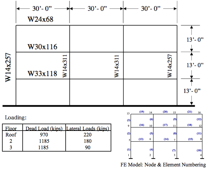
OpenSees Basic Examples (H1: 弾性フレーム解析) 例題

   Elastic Frame Example　参照


例題では、下図の様な構造の弾性フレーム(H形鋼：鉄骨Wフランジ）を使っています。
そのため、Ｚ軸の慣性モーメント や断面積はきまっています

H形鋼のアメリカでの仕様書は、以下のサイトを見ると、出ています。
http://www.webcivil.com/readusshapew.aspx

座標の軸については、赤がH形鋼の座標、青がOpenSeesの計算で使用する座標です。
そのため、OpenSeesのElement(要素)設定の時に使用する、Z軸の慣性モーメントは、
H形鋼の仕様書の Ix を使用する事になります。

この例題で使用する鉄骨Wフランジの値です。

In x lb/ft	断面積 (Area) in2	Z軸の慣性 モーメント  (Ix) in4	X軸の慣性 モーメント  (Iy) in4	d (in)	bf (in)	tf (in)	tw (in)
W33x118	34.7	5900	187	32.9	11.5	0.74	0.55
W30x116	34.2	4930	164	30	10.5	0.85	0.565
W24x68	20.1	1830	70.4	23.37	8.965	0.585	0.415
W14x257	75.6	3400	1290	16.38	15.995	1.89	1.175
W14x331	91.4	4330	1610	17.12	16.23	2.26	1.41

例題はこの図のとおりです
Node(節点）黒数字
Element(要素）青カッコ数字
を以下の様に設定し、節点1,2,3,4は固定されています

次のページ　→
Basic Examples  (Elastic Frame)　
解説(Node,Element)

Opensees コマンド　日本語解説　： 目次

夏休みのお知らせ

OpenSeesファンの皆様

このブログを見ていただきましてありがとうございます。毎週１，２ページの投稿を目標にしておりますが、アルバイト先の研究室の論文サマリを急いで英訳しなければいけないこともあり（汗）、本日より８月末まで夏休みを取らせていただきます。

目次ページにありますとおり、次回は
Basic example manual　の
Elastic Frame Example
に取り組む予定です。

Googleさんの統計によりますと
このブログを開設してから 約２か月、本日まで1200ビュー(＊）、約100人ぐらいの方に見ていただいているようです。
また、日本ばかりでなく、アメリカ、ロシア、ドイツ、ウクライナercの国の方も閲覧しているようです。ありがとうございます。

夏休み後もまったりと追記していきますので、よろしくお願いします。

Innovativeな建物がたくさんできますように！
2014/7/25 Satoko Toengawa

(*)Tonegawaが閲覧したビュー数、リダイレクトしたビュー数は除いた数字です

OpenSees Basic Examples (A3: 基本的なトラス解析) 解析結果

Truss example(ここ)で作成した、Truss.Tcl ファイル内の
OpenSeesコマンドを実行すると、以下の様な画面が表示されます。

Node3 について
座標は　(72,96)
変位は　0.530093 -0.177894
速度は　なし
外部からの力は　X方向100 Y方向 -50


また、 下記コマンド

recorder Node -file TrussNode.txt -time -node 4 -dof 1 2 disp

recorder Element -file TrussEleGlobal.txt -time -ele 1 2 3 forces
recorder Element -file TrussEleLocal.txt -time -ele 1 2 3  basicForces

から、テキストファイル
TrussNode.txt
TrussEleGlobal.txt
TrussEleLocal.tct
として出力されます


そして、下記コマンド
print element

から、テキストファイル
element
として出力されます

<TrussNode.txt>

time	Node4での	Node4での
	X方向の変位	Y方向の変位
1	0.530093	-0.177894

<TrussEleGlobal.txt>
全体座標系

	Element 1
	Node1		Node4
time	X方向の力	Y 方向の力	X方向の力	Y 方向の力
1	-26.3611	-35.1482	26.3611	35.1482
	Element 2
	Node2		Node4
	X方向の力	Y 方向の力	X方向の力	Y 方向の力
	-34.5278	46.0371	34.5278	-46.037
	Element 3
	Node3		Node4
	X方向の力	Y 方向の力	X方向の力	Y 方向の力
	-39.1111	39.1111	39.1111	-39.111

<TrussEleLocal.txt>
局所座標系（部材座標系)

time	Element 1軸力	Element 2　軸力	Element 3　軸力
1	43.9352	-57.5463	-55.3114

Opensees コマンド　日本語解説　： 目次