OpenSees Blog 日本語 目次

最初に「このブログをみるためのガイド」をご覧ください。

Update中OpenSees コマンド 日本語解説 の 目次 OpenSeesコマンド はじめての方は「ここから
このblogで使用しているOpenSeesコマンド集は「ここ」 Update中
OpenSees のソースコード 解析に挑戦してみる 目次最初のページは「ソースコードのダウンロードとビルド」
Appendix:C言語での 「有限要素法における平面トラスの解析」目次最初のページは「Microsoft Visual Studioの導入方法」


目次の中で、更新したページにはNewがついています

このブログ内の単語を検索したい場合は、左上OpenSeesロゴの上に検索窓から検索できます。


2023年4月21日金曜日

2018年4月18日水曜日

Kindle 本 Version 1.1  出しました


日本版


US版  Written in Japanese

修正/追加点は、以下の通りです
V1.0 でありました単位の間違いの修正
PowerShellでOpenSeesを実行する方法
   Microsoft: 最新のWindows 10リリースで「コマンドプロンプト」を削除する方向もある、ということですので、DOSコマンドプロンプトの代わりに、PowerShellでOpenSeesを実行する方法を記載

よろしくお願いします!

2017年11月16日木曜日

OpenSees Basic Examples ( D5: 2階建て単スパンフレームでの固有値解析) 解析結果

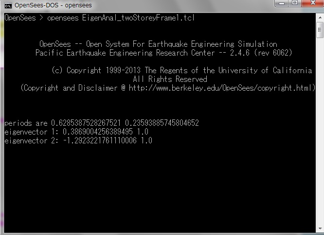
2階建て単スパンフレームでの固有値解析(ここ)で作成した、EigenAnal_twoStoreyFrame1.tclファイル内の OpenSeesコマンドを実行すると、以下の様な画面が表示されます。


1次の固有周期は 0.6285387528267521
2次の固有周期は 0.23593885745804652

このデータは、modesフォルダーの中のPeriods.txtの中にもあります

1次の固有振動モード(固有ベクトル)eigenvector は {0.3869004256389495 1.0}
2次の固有振動モード(固有ベクトル)eigenvector は {-1.2923221761110006 1.0}


また、
1次モード、2次モードのx,yの1次、2次の振動モード形を
OpenSeesによりプロットした結果は以下の様になります。

このグラフのデータは、modesフォルダーの中のmode1.outとmode2.outにあります。

Node1 Node2
x y θ x y θ
mode1 0 0 0 0 0 0
mode2 0 0 0 0 0 0

Node3 Node4
x y θ x y θ
mode1 0.666844 0.00224274 -0.00599676 0.666844 #VALUE! -0.00599676
mode2 1.21874 -0.00138942 -0.00256026 1.21874 0.00138942 -0.00256026

Node5 Node6
x y θ x y θ
mode1 1.72355 0.00297706 -0.0058452 1.72355 -0.00297706 -0.0058452
mode2 -0.94306 -0.00342779 0.0161851 -0.94306 0.00342779 0.0161851


Opensees コマンド 日本語解説 : 目次


2017年2月6日月曜日

OpenSees Basic Examples ( D4: 2階建て単スパンフレームでの固有値解析) コマンドサマリ


Basic Examples ( 2階建て単スパンフレームでの固有値解析)   解説
のコマンドのサマリは以下の通りです。

このコマンドを ファイル名 EigenAnal_twoStoreyFrame1.tcl として、テキストフォーマットで作成し、
OpenSeesの起動環境 で 起動しているOpenSees のコマンドラインに

OpenSees EigenAnal_twoStoreyFrame1.tcl  <Enter>

と打ち込んで、実行します。

-----EigenAnal_twoStoreyFrame1.tcl 始まり ------

# Eigen analysis of a two-storey one-bay frame; Example 10.5 from "Dynamics of Structures" book by Anil Chopra

# units: kips, in, sec

#       Vesna Terzic, 2010

#delete all previosly constructed objects
wipe;    

#set input variables
#--------------------

#mass
set m  [expr 100.0/386.0]

#number of modes
set numModes 2

#material
set A 63.41
set I 320.0
set E 29000.0

#geometry
set L 240.
set h  120.

# create data directory
file mkdir modes;

# define the model
#---------------------------------
#model builder
model BasicBuilder -ndm 2 -ndf 3

# nodal coordinates:
node 1   0.  0. ;
node 2   $L  0. ;
node 3   0.  $h ;
node 4   $L  $h ;
node 5   0.  [expr 2*$h];
node 6   $L  [expr 2*$h];

# Single point constraints -- Boundary Conditions
fix 1 1 1 1;
fix 2 1 1 1;

# assign mass
mass 3 $m 0. 0. ;
mass 4 $m 0. 0. ;
mass 5 [expr $m/2.] 0. 0. ;
mass 6 [expr $m/2.] 0. 0. ;

# define geometric transformation:
set TransfTag 1;
geomTransf Linear $TransfTag ;

# define elements:
# columns
element elasticBeamColumn 1 1 3 $A $E [expr 2.*$I] $TransfTag;
element elasticBeamColumn 2 3 5 $A $E $I           $TransfTag;
element elasticBeamColumn 3 2 4 $A $E [expr 2.*$I] $TransfTag;
element elasticBeamColumn 4 4 6 $A $E $I           $TransfTag;
# beams
element elasticBeamColumn 5 3 4 $A $E [expr 2.*$I] $TransfTag;
element elasticBeamColumn 6 5 6 $A $E $I           $TransfTag;

# record eigenvectors
#----------------------
for { set k 1 } { $k <= $numModes } { incr k } {
    recorder Node -file [format "modes/mode%i.out" $k] -nodeRange 1 6 -dof 1 2 3  "eigen $k"
}

# perform eigen analysis
#-----------------------------
set lambda [eigen  $numModes];

# calculate frequencies and periods of the structure
#---------------------------------------------------
set omega {}
set f {}
set T {}
set pi 3.141593

foreach lam $lambda {
lappend omega [expr sqrt($lam)]
lappend f [expr sqrt($lam)/(2*$pi)]
lappend T [expr (2*$pi)/sqrt($lam)]
}

puts "periods are $T"

# write the output file cosisting of periods
#--------------------------------------------
set period "modes/Periods.txt"
set Periods [open $period "w"]
foreach t $T {
puts $Periods " $t"
}
close $Periods

# record the eigenvectors
#------------------------
record

# create display  for mode shapes
#---------------------------------
#                 $windowTitle $xLoc $yLoc $xPixels $yPixels
recorder display "Mode Shape 1"  10    10     500      500     -wipe
prp $h $h 1;                                         # projection reference point (prp); defines the center of projection (viewer eye)
vup  0  1 0;                                         # view-up vector (vup)
vpn  0  0 1;                                         # view-plane normal (vpn)  
viewWindow -200 200 -200 200;                        # coordiantes of the window relative to prp
display -1 5 20;                                     # the 1st arg. is the tag for display mode (ex. -1 is for the first mode shape)
                                                     # the 2nd arg. is magnification factor for nodes, the 3rd arg. is magnif. factor of deformed shape
recorder display "Mode Shape 2" 10 510 500 500 -wipe
prp $h $h 1;
vup  0  1 0;
vpn  0  0 1;
viewWindow -200 200 -200 200
display -2 5 20

# get values of eigenvectors for translational DOFs
#---------------------------------------------------
set f11 [nodeEigenvector 3 1 1]
set f21 [nodeEigenvector 5 1 1]
set f12 [nodeEigenvector 3 2 1]
set f22 [nodeEigenvector 5 2 1]
puts "eigenvector 1: [list [expr {$f11/$f21}] [expr {$f21/$f21}] ]"
puts "eigenvector 2: [list [expr {$f12/$f22}] [expr {$f22/$f22}] ]"

after 10000

----- EigenAnal_twoStoreyFrame1.tcl 終わり ------


次のページ →
OpenSees Basic Examples ( D4: 2階建て単スパンフレームでの固有値解析) 解析結果


Opensees コマンド 日本語解説 : 目次

2017年1月25日水曜日

2017年1月18日水曜日

OpenSees Basic Examples ( D2: 2階建て単スパンフレームでの固有値解析) 解説(Node, Element)


0)必要となる数字をシンボルに代入しておき、実行環境を生成します

#input
set m  [expr 100.0/386.0]
set numModes 2      # 解析する固有値モードの数

#material
set A 63.41    # Element 1,2,3,4,5,6の断面積
set I 320.0       #Element 2,4,6の慣性モーメント
set E 29000.0  # ヤング率

#geometry
set L 240.
set h  120.

# create data directory "mkdir"のディレクトリを生成します
file mkdir modes; 


1)Model, Node(節点), Element(要素)の設定
解析する時の、次元、節点(Node)、要素(Element)の
Opensees のコマンドは、以下の通りです。

1.1) 2次元、自由度3 で、解析するよう設定します
model BasicBuilder [次元数] [自由度数] 

model BasicBuilder -ndm 2 -ndf 3

(参照ページはここ

1.2) Node(節点) の 座標を設定します
Node [ nodeの番号 ] [ x座標] [y座標] -mass [節点質量(自由度の第1成分:u )]
[節点質量(自由度の第2成分:v )] [節点質量(自由度の第3成分:θ )]

$がついた変数は、0)の所で定義したシンボルの数字がはいります。


# nodal coordinates:
node 1   0.  0. ;
node 2   $L  0. ;
node 3   0.  $h ;
node 4   $L  $h ;
node 5   0.  [expr 2*$h];    #  = 2 x h 
node 6   $L  [expr 2*$h];       #  = 2 x h 

1.3) Nodeのどこを固定するかを設定します
ここでは、nodeの1と2を固定します。

fix [ nodeの番号 ] [ uの固定の定義]  [ vの固定の定義]  [ θの固定の定義] 
0: 固定されていない
1: 固定されている


# Single point constraints -- Boundary Conditions
fix 1 1 1 1;
fix 2 1 1 1;


(参照ページはここ

1.4) Nodeの質量の定義

Nodeの質量を指定します。

Node3,4  Node5,6 の水平方向のみの質量が定義されています

mass [ nodeの番号 ] [ uの質量]  [ vの質量]  θ回転慣性質量] 


# assign mass
mass 3 $m 0. 0. ;
mass 4 $m 0. 0. ;
mass 5 [expr $m/2.] 0. 0. ;
mass 6 [expr $m/2.] 0. 0. ;

(参照ページはここ

1.5) 座標変換の定義

geomTransf [座標変換の方法] [座標変換方法のID]


# define geometric transformation:
set TransfTag 1;
geomTransf Linear $TransfTag ;


(参照ページはここ


1.6) Element(要素)を設定します。

Element コマンド の中の elasticBeamColum を使用します。

element elasticBeamColumn [ elementの番号 ] [ 片方のnode番号] [片方のnode番号] [ 断面積] [ヤング率] [Z軸の慣性モーメント] [座標変換方法のID]


# define elements:
# columns
element elasticBeamColumn 1 1 3 $A $E [expr 2.*$I] $TransfTag;
element elasticBeamColumn 2 3 5 $A $E $I           $TransfTag;
element elasticBeamColumn 3 2 4 $A $E [expr 2.*$I] $TransfTag;
element elasticBeamColumn 4 4 6 $A $E $I           $TransfTag;
# beams
element elasticBeamColumn 5 3 4 $A $E [expr 2.*$I] $TransfTag;
element elasticBeamColumn 6 5 6 $A $E $I           $TransfTag;


(参照ページはここ


次のページ →
OpenSees Basic Examples ( D3: 2階建て単スパンフレームでの固有値解析)) 解説(固有値解析)


Opensees コマンド 日本語解説 : 目次

2017年1月12日木曜日

OpenSees Basic Examples ( D1: 2階建て単スパンフレームでの固有値解析) 例題


  Eigen analysis of a two-storey one-bay frame 参照


例題は、下図の通りです。
Chopra教授の "Dynamic of Structures" からの例題です
10章  Free Vibration  part A Natural Vibration Frequencies and modes 10.4章 Orthogonality of modes

柱、桁の軸変形は無視、軸力の影響も無視した、理想的な形状として定義しています
軸と桁の断面積、Z軸慣性モーメント、ヤング率は同じ状態としています。

単位は in, kips です


NodeとElementの場所は、下図のとおりです


h = 120
L = 2h = 240

m = 100.0/386.0 (集中質量)

解析する固有値モードの数 2

次のページ →
OpenSees Basic Examples ( D1: 2階建て単スパンフレームでの固有値解析) 解説(Node, Element)


Opensees コマンド 日本語解説 : 目次


2016年12月24日土曜日

PowerShell で OpenSeesコマンドを実行するには


2016/12/24 メリークリスマス

http://business.newsln.jp/news/201612072350480000.html
Microsoft: 最新のWindows 10リリースで「コマンドプロンプト」を削除

という記事をみつけましたので、DOSコマンドプロンプトの代わりに、PowerShellでOpenSeesを実行することができるだろうか、ということで調査してみました。

PowerShellでOpenSeesを実行するには、以下の2つの方法があることを確認しました!

---------------------------------------------------------

PowerShellでの問題は、WindowsのpathをPowerShell 上で設定しなければいけない事

PowerShell上でスクリプトを実行させるときは、実行ポリシーを変更しなければいけない事
に注意しなければいけません。

<方法1>

1) PowerShell を立ち上げる

2) OpenSeesのTCLファイルがあるディレクトリへ移動する

3) $env:path += ";C:\Tcl\bin;C:\OpenSees\tools;"
を実行

4)  $env:path
を実行。OpenSeesとTclのディレクトリにパスが通っていることを確認する

5) OpenSees XXXXX.tcl
OpenSeesコマンドが記述されているtcl ファイルをOpenSeesコマンドで実行

方法1では、pathの設定のためのコマンドが長いので、いちいちタイピングするのは面倒です。
そのため、この部分とOpenSeesの実行を一つのPowerShellスクリプトとして実行することによって、タイプするコマンドを少なくする方法が<方法2>です。

<方法2>

0) 前準備として、
OpenSeesのTCLファイルがあるディレクトリで、下記のファイルを作成する

a) envPS.bat ファイル

@echo off
echo OpenSeesを実行しています
powershell -NoProfile -ExecutionPolicy Unrestricted .\envPS-OS  %1
echo 実行終了


b) envPS-OS.ps1 ファイル

$env:path += ";C:\Tcl\bin;C:\OpenSees\tools;"
OpenSees $Args[0]

1) PowerShell を立ち上げる

2) OpenSeesのTCLファイルがあるディレクトリへ移動する

3) .\envPS  XXXXX.tcl
を実行

例えば
truss-test.tcl を実行するには

.\envPS truss-test.tcl

になり、
実行結果は以下のとおりです


2016年12月21日水曜日

OpenSees Basic Examples (F9:2D 梁への固体動力学問題) 解析結果

2D 梁への固体動力学問題(ここ)で作成した、Ex6_4.tclファイルの OpenSeesコマンドを実行すると、以下の様な画面が表示されます。


コンピュータのディスプレイ画面の右上に
OpenSees Basic Examples (F6::2D 梁への固体動力学問題) シュミレーション結果の画像表示
で指定した画像が動画として表示されます。

上辺の真ん中のNode (77) と底辺の真ん中のNode(9) に外力を加えてから、レイリー減衰する様子が動画としてみることができます。


外力を加えたNode
I1 :  底辺の真ん中  → 9
I2 : 上辺の真ん中  → 77

固定点
1 : 左下
bn : 右下 → 17

また、 下記コマンド

# define the recorder
#---------------------
recorder Node -file Data/Node.txt -time -node $l1 -dof 1 2 disp

から、Dataフォルダーに、テキストファイル
Node.txt
が出力されます

底辺の真ん中のNode(9) のY方向の変位を記録しています。

time Node9でのY方向の変位
1 -0.0408198
2 -0.0816397
3 -0.12246
4 -0.163279
5 -0.204099
6 -0.244919
7 -0.285739
8 -0.326559
9 -0.367379
10 -0.408198
0.5 -0.397438
1 -0.377159
1.5 -0.357813
2 -0.333959
2.5 -0.305644
  :
  :
      :
      :
745 0.00546469
745.5 0.00631982
746 0.00708078
746.5 0.00773715
747 0.00828008
747.5 0.00870237
748 0.00899857
748.5 0.00916506
749 0.00920007
749.5 0.00910375
750 0.00887808

時間が10秒の後、0.5秒になっていますが、これは、

OpenSees Basic Examples (F7::2D 梁への固体動力学問題) レイリー減衰を追加しての解析設定
で、測定時間を0.0 秒にリセットしたためです。
setTime 0.0

そのため、実際は、0.5秒ではなく、10.5秒、 11.0秒・・・となります。

これをグラフにしたものは以下のとおりです。


Node9は、外力を加えたNodeであり、また、固定されているNode同士の中間地点であるので、一番レイリー減衰を顕著にみることができます。


2016年12月14日水曜日

OpenSees Basic Examples (F8:2D 梁への固体動力学問題) コマンドサマリ


Basic Examples (2D 梁への固体動力学問題)   解説
のコマンドのサマリは以下の通りです。

このコマンドを ファイル名 EigenAnal_twoStoreyFrame1.tcl として、テキストフォーマットで作成し、
OpenSeesの起動環境 で 起動しているOpenSees のコマンドラインに

OpenSees EigenAnal_twoStoreyFrame1.tcl  <Enter>

と打ち込んで、実行します。

----- EigenAnal_twoStoreyFrame1.tcl 始まり ------
# Eigen analysis of a two-storey one-bay frame; Example 10.5 from "Dynamics of Structures" book by Anil Chopra

# units: kips, in, sec

#       Vesna Terzic, 2010

#delete all previosly constructed objects
wipe;    

#set input variables
#--------------------

#mass
set m  [expr 100.0/386.0]

#number of modes
set numModes 2

#material
set A 63.41
set I 320.0
set E 29000.0

#geometry
set L 240.
set h  120.

# create data directory
file mkdir modes;

# define the model
#---------------------------------
#model builder
model BasicBuilder -ndm 2 -ndf 3

# nodal coordinates:
node 1   0.  0. ;
node 2   $L  0. ;
node 3   0.  $h ;
node 4   $L  $h ;
node 5   0.  [expr 2*$h];
node 6   $L  [expr 2*$h];

# Single point constraints -- Boundary Conditions
fix 1 1 1 1;
fix 2 1 1 1;

# assign mass
mass 3 $m 0. 0. ;
mass 4 $m 0. 0. ;
mass 5 [expr $m/2.] 0. 0. ;
mass 6 [expr $m/2.] 0. 0. ;

# define geometric transformation:
set TransfTag 1;
geomTransf Linear $TransfTag ;

# define elements:
# columns
element elasticBeamColumn 1 1 3 $A $E [expr 2.*$I] $TransfTag;
element elasticBeamColumn 2 3 5 $A $E $I           $TransfTag;
element elasticBeamColumn 3 2 4 $A $E [expr 2.*$I] $TransfTag;
element elasticBeamColumn 4 4 6 $A $E $I           $TransfTag;
# beams
element elasticBeamColumn 5 3 4 $A $E [expr 2.*$I] $TransfTag;
element elasticBeamColumn 6 5 6 $A $E $I           $TransfTag;

# record eigenvectors
#----------------------
for { set k 1 } { $k <= $numModes } { incr k } {
    recorder Node -file [format "modes/mode%i.out" $k] -nodeRange 1 6 -dof 1 2 3  "eigen $k"
}

# perform eigen analysis
#-----------------------------
set lambda [eigen  $numModes];

# calculate frequencies and periods of the structure
#---------------------------------------------------
set omega {}
set f {}
set T {}
set pi 3.141593

foreach lam $lambda {
lappend omega [expr sqrt($lam)]
lappend f [expr sqrt($lam)/(2*$pi)]
lappend T [expr (2*$pi)/sqrt($lam)]
}

puts "periods are $T"

# write the output file cosisting of periods
#--------------------------------------------
set period "modes/Periods.txt"
set Periods [open $period "w"]
foreach t $T {
puts $Periods " $t"
}
close $Periods

# record the eigenvectors
#------------------------
record

# create display  for mode shapes
#---------------------------------
#                 $windowTitle $xLoc $yLoc $xPixels $yPixels
recorder display "Mode Shape 1"  10    10     500      500     -wipe
prp $h $h 1;                                         # projection reference point (prp); defines the center of projection (viewer eye)
vup  0  1 0;                                         # view-up vector (vup)
vpn  0  0 1;                                         # view-plane normal (vpn)    
viewWindow -200 200 -200 200;                        # coordiantes of the window relative to prp
display -1 5 20;                                     # the 1st arg. is the tag for display mode (ex. -1 is for the first mode shape)
                                                     # the 2nd arg. is magnification factor for nodes, the 3rd arg. is magnif. factor of deformed shape
recorder display "Mode Shape 2" 10 510 500 500 -wipe
prp $h $h 1;
vup  0  1 0;
vpn  0  0 1;
viewWindow -200 200 -200 200
display -2 5 20

# get values of eigenvectors for translational DOFs
#---------------------------------------------------
set f11 [nodeEigenvector 3 1 1]
set f21 [nodeEigenvector 5 1 1]
set f12 [nodeEigenvector 3 2 1]
set f22 [nodeEigenvector 5 2 1]
puts "eigenvector 1: [list [expr {$f11/$f21}] [expr {$f21/$f21}] ]"
puts "eigenvector 2: [list [expr {$f12/$f22}] [expr {$f22/$f22}] ]"


after 10000

----- EigenAnal_twoStoreyFrame1.tcl 終わり ------

 次のページ → 
OpenSees Basic Examples (F9::2D 梁への固体動力学問題) 解析結果

2016年12月7日水曜日

OpenSees Basic Examples (F7:2D 梁への固体動力学問題) レイリー減衰を追加しての解析設定


12) レイリー減衰を追加しての解析設定

レコーダー、外力の設定 で設定した外力を加えた後、レイリー減衰により、減衰をさせ、
減衰中のデータを解析するための設定を行い、シュミレーションを行います。

rayleigh [質量マトリクス係数] [瞬間剛性マトリクス係数] [初期剛性マトリクス係数] [committed stiffness matrix係数]

rayleigh コマンドの詳細については、「Getting started 地震波データの入力・解析」 での 「外力の設定-レイリー減衰の指定」  を参照してください

# ---------------------------------------
# Create and Perform the dynamic analysis
# ---------------------------------------
#define damping
rayleigh 0. 0. 0. [expr 2*0.02/sqrt([eigen 1])];

wipeAnalysisコマンドで、いままで使っていた解析設定をすべてリセットします

setTimeコマンドで、解析開始時刻を0.0 にリセットします

removeコマンドで、かけていた外力をなくします

# Remove the static analysis & reset the time to 0.0
wipeAnalysis
setTime 0.0

# Now remove the loads and let the beam vibrate
remove loadPattern 1

かかっていた外力がなくなった状態でレイリー減衰した時のシュミレーションを行うための解析の設定を行います。
ほぼ、
OpenSees Basic Examples (F5::2D 梁への固体動力学問題)解析の設定
と同じものを使用しています。

test EnergyIncr [耐性基準] [もし収束判定がエラーだった場合、再試行する回数] [判定結果の表示方法の指定]

注)  [判定結果の表示方法の指定] は 「何も表示しない」(=0) と指定している

# Convergence test
#              tolerance maxIter displayCode
test EnergyIncr 1.0e-12    10         0


方程式の解法は、Newton法を使用します。(algorithmコマンド)

algorithm Newton


有限要素法解析で生成される係数行列での疎行列を解く場合の、行列の再配列方法は逆カットヒル・マキー法 (Reverse Cuthill–McKee algorithm ,RCM)を使用する (numbererコマンド)

numberer RCM

制約のついた非線形問題を制約なし問題に変換して解く変換法は、Plainを使用する(constraintsコマンド)

constraints Plain

analysisコマンド で Transient と指定しています。

analysis [解析タイプ] Static / Transient / VariableTransient
analysis Transient

Transientでのニューマーク法を使用します。Newmark コマンドの説明は ここ にあります。

integrator Newmark [ γ値 ] [ β値 ]

ここでは
γ値 0.5  β値 0.25
ニューマーク法の定加速度法
を使用しています

integrator Newmark 0.5 0.25

線形連立方程式)の解法のために使用するプログラムは、LAPACKライブラリ(DGBSV)の実帯連立一次方程式を使用する (systemコマンド)
system BandGeneral

解析設定が終わった時点でシュミレーションを実行します
analyze [実行する回数] [増加させる秒数]

# Perform the transient analysis (50 sec)
analyze 1500 0.5

まとめると、以下の通り。

# ---------------------------------------
# Create and Perform the dynamic analysis
# ---------------------------------------
#define damping
rayleigh 0. 0. 0. [expr 2*0.02/sqrt([eigen 1])];

# Remove the static analysis & reset the time to 0.0
wipeAnalysis
setTime 0.0

# Now remove the loads and let the beam vibrate
remove loadPattern 1

# Create the transient analysis
test EnergyIncr 1.0e-12 10 0
algorithm Newton
numberer RCM
constraints Plain
integrator Newmark 0.5 0.25
system BandGeneral
analysis Transient

# Perform the transient analysis (50 sec)
analyze 1500 0.5


 次のページ → 
OpenSees Basic Examples (F8::2D 梁への固体動力学問題) コマンドサマリ

2016年11月30日水曜日

OpenSees Basic Examples (F6:2D 梁への固体動力学問題) シュミレーション結果の画像表示

11) シュミレーション結果の画像表示


行うシュミレーションの結果をグラッフィック表示させます。

最初に、表示するWindowsについて設定します。
recorder display "[表示するWindowのタイトル]" [表示するWindowの左上の位置(x)]  [表示するWindowの左上の位置(y)] [表示するWindowの大きさ(幅)] [表示するWindowの大きさ(高さ)] -wipe 

ここでの「表示するWindowの左上」は、コンピュータ画面の左上からの位置になります。
また、単位はピクセル(画素数)です。

# -------------------------------------
# create display for transient analysis
#--------------------------------------
#                    $windowTitle       $xLoc $yLoc $xPixels $yPixels
recorder display "Simply Supported Beam" 10     10      800     200    -wipe

Projector reference point (prp) 投影基準点
View-up vector (vup)
View-plane normal (vpn)
View Reference Point (vrp)
は、コンピュータグラッフィックスについての用語で、下図の様な定義となります。
詳細については、Viewpoint Projections and Specifications に記載されています。


prp 20 5.0 1.0;
 # projection reference point (prp); defines the center of projection (viewer eye)

vup  0  1 0;                                    
  # view-up vector (vup)

vpn  0  0 1;                                    
  # view-plane normal (vpn)

グラッフィックとして表示する座標範囲は、viewWindowコマンドで指定します。

viewWindow [ViewPlain上でのu方向左端]  [ViewPlain上でのu方向右端]  [ViewPlain上でのv方向下端]   [ViewPlain上でのv方向上端] 

viewWindow -30 30 -10 10;                    
  # coordiantes of the window relative to prp

最後に表示させる為のdisplayコマンドを設定する。

display [表示の見せ方] [拡大係数] [変形形状の強さ]

2階建てフレームでの固有値解析 では、[表示の見せ方] は、マイナスの値をとり、絶対値の値がn次固有モードを表したが、今回は 10を設定しているので、固有モードではないので、注意してください。

display 10 0 5;                                
  # the 1st arg. is the tag for display mode
  # the 2nd arg. is magnification factor for nodes, 
 # the 3rd arg. is magnif. factor of deformed shape

まとめると、以下の通り。

# -------------------------------------
# create display for transient analysis
#--------------------------------------
#                    $windowTitle       $xLoc $yLoc $xPixels $yPixels
recorder display "Simply Supported Beam" 10     10      800     200    -wipe
prp 20 5.0 1.0;                                
  # projection reference point (prp); defines the center of projection (viewer eye)
vup  0  1 0;                                      
  # view-up vector (vup)
vpn  0  0 1;                                      
  # view-plane normal (vpn)  
viewWindow -30 30 -10 10;                      
  # coordiantes of the window relative to prp
display 10 0 5;                                  
  # the 1st arg. is the tag for display mode
  # the 2nd arg. is magnification factor for nodes, the 3rd arg. is magnif. factor of deformed shape


 次のページ → 
OpenSees Basic Examples (F7::2D 梁への固体動力学問題) レイリー減衰を追加しての解析設定

2016年11月15日火曜日

ありがとうございます

OpenSees ユーザーズガイド: インストールと初めての使い方(Kindle版)
を出してから半月ほどになりました。

ご購入していただいた方、こちらではお名前等なにもわからないのが残念ですが、大変ありがとうございます。


本日kindle shopを見てみましたら、インテリアデザインのカテゴリーで一位になっていました。おそらく瞬間的なのでしょうが、記念にとったスクリーンショットが、こちらです。


この本が、プログラムを使うにあたっての助けになれば幸いです。
よろしくお願い致します。

2016年11月9日水曜日

OpenSees Basic Examples (F5:2D 梁への固体動力学問題)解析の設定


10)解析の設定

9)外力の設定で指定した荷重をかけている間の解析について設定しています。

解析する時の、連立方程式の解き方の手法などを設定します。
各コマンドの説明は、「OpenSeesコマンド集」を参照してください

解析は、Static で行い(analysis コマンド)、解析の間隔は1secから10secまで、1secづつ行う。(Integratorコマンド) 

analysis [解析タイプ] Static / Transient / VariableTransient

# Type of analysis analysis
analysis Static

integrator LoadControl  [解析する時間間隔] [解析を行う時間間隔の頻度間隔] [初期時間] [ 最終時間] 

(注) [解析を行う時間間隔の頻度間隔] は、
1がセットされた場合は、(初期値が1secの場合) 1, 2, 3, 4, 5sec となる
2がセットされた場合は、(初期値が1secの場合) 1, 3, 7, 15sec となる

# Load control with variable load steps
#                      init Jd min max
integrator LoadControl 1.0   1 1.0 10.0

連立方程式を解く時の収束判定は、エネルギーの変化をもとにして行う(testコマンド)

test EnergyIncr [耐性基準] [もし収束判定がエラーだった場合、再試行する回数] [判定結果の表示方法の指定]

注)  [判定結果の表示方法の指定] は 「何も表示しない」(=0) と指定している

# Convergence test
#              tolerance maxIter displayCode
test EnergyIncr 1.0e-12    10         0

方程式の解法は、Newton法を使用します。(algorithmコマンド)

# Solution algorithm
algorithm Newton

有限要素法解析で生成される係数行列での疎行列を解く場合の、行列の再配列方法は逆カットヒル・マキー法 (Reverse Cuthill–McKee algorithm ,RCM)を使用する (numbererコマンド)

# DOF numberer
numberer RCM

制約のついた非線形問題を制約なし問題に変換して解く変換法は、Plainを使用する(constraintsコマンド)

# Cosntraint handler
constraints Plain

線形連立方程式)の解法のために使用するプログラムは、LAPACKライブラリ(DPOSV)の実対称正定値連立一次方程式を使用する (systemコマンド)

# System of equations solver
system ProfileSPD

解析設定が終わった時点で、9)外力の設定で指定した荷重をかけて10secシュミレーションします。

analyze [実行する回数] 

まとめると、以下の通り。

# --------------------------------------------------------------------
# Start of static analysis (creation of the analysis & analysis itself)
# --------------------------------------------------------------------

# Load control with variable load steps
#                      init Jd min max
integrator LoadControl 1.0   1 1.0 10.0

# Convergence test
#              tolerance maxIter displayCode
test EnergyIncr 1.0e-12    10         0

# Solution algorithm
algorithm Newton

# DOF numberer
numberer RCM

# Cosntraint handler
constraints Plain

# System of equations solver
system ProfileSPD

# Type of analysis analysis
analysis Static

# Perform the analysis
analyze 10

# --------------------------
# End of static analysis
# --------------------------


 次のページ → 
OpenSees Basic Examples (F6::2D 梁への固体動力学問題) シュミレーション結果の画像表示

2016年11月4日金曜日

OpenSees Basic Examples (F4:2D 梁への固体動力学問題) レコーダー、外力の設定


8)解析結果を記録するレコーダーの設定
Node(節点)の解析結果を記録するためのファイル名、Node番号を設定します

recorder Node -file [ 出力ファイル名 ] -time(時間を基準として記録) -node[記録したいNode番号] -dof[記録したい自由度] disp(相対的な変位を出力) 

Node 9 での X,Y成分における変位を時間ごとに記録します。

# define the recorder
#---------------------
recorder Node -file Data/Node.out -time -node $l1 -dof 2 disp

$I1 は、ここで定義された 値が入ります。
I1 は、底辺の真ん中  → 9

Data/Node.out
の表記は、OpenSeesを動作させているフォルダーの下に、Dataというフォルダーを作成した上で、ファイル名 Node.out  に 出力結果を書きだします。

(参照ページはここ)

9)外力の設定
この構造物に加える外力(緑の部分)を設定します。

$I1、$I2 は、ここで定義された 値が入ります。
I1 は、底辺の真ん中  → 9
I2 は、上辺の真ん中  → 77

pattern Plain [Loadの通し番号] Linear  {
     load [Node番号] [自由度の1番目に対してかける力(X方向)] [ 自由度の1番目に対してかける力(Y方向)] 

      [ 自由度の3番目に対してかける力(θ方向)]
}

時間ごとに一定に、Node9 と Node77 に対して、Y方向 -1.0 の荷重をかけます。

# define load pattern
#---------------------
pattern Plain 1 Linear {
load $l1 0.0 -1.0
load $l2 0.0 -1.0


 次のページ → 
OpenSees Basic Examples (F5::2D 梁への固体動力学問題)解析の設定

Opensees コマンド 日本語解説 : 目次

2016年10月6日木曜日

OpenSees ユーザーズガイド: インストールと初めての使い方 Kindle版


OpenSees ユーザーズガイド: インストールと初めての使い方 Kindle版


出荷を開始しました。

Blogにぽちぽち書いていた内容が、古くなっておりましたので、新しいデータと2016年10月現在の情報に書き直したものを、まとめました。

OpenSeesのInstall 方法、はじめての使い方を解説している Getting stared の内容の説明と、実際にOpenSeesで動作させた出力結果、および、”PEER Ground Motion Database”のデータベースの使い方 おもに「コンピュータの使い方」の視点からの解説しています。約100ページ。

ご使用いただけましたら幸いです。


2016年8月27日土曜日

現在 公開停止中です

この数週間、あるIPアドレスが示す国から、異常な数の閲覧数が、数日続いて起こったため、
しばらく、最新の情報と目次以外を残して、公開を止めています。

もし特別なご希望などがありましたら、メール、コメントいただければ対応いたします

よろしくご理解お願いします
管理者2016年 8月1日

しばらく時間がたったので、一部、もとに戻しました。
管理者2016年9月4日


2016年7月20日水曜日

OpenSees Basic Examples (F3:2D 梁への固体動力学問題)Node(節点), Element(要素)の設定


6) Node(節点), Element(要素)の設定

下図の様な構造物を設定します。


構造物は、メッシュで設定されていますが、
X方向、Y方向それぞれのブロックの数は、Xは4つ、Yは16つです。

# set up the number of elements in x (nx) and y (ny) direction
set nx 16; # NOTE: nx MUST BE EVEN FOR THIS EXAMPLE
set ny 4

重要な部分のNodeの番号をシンボルとして代入しておきます。
bn は、右下 → 17
I1 は、底辺の真ん中  → 9
I2 は、上辺の真ん中  → 77

# define numbering of node at the left support (bn), and the two nodes at load application (l1, l2)
set bn [expr $nx + 1]
set l1 [expr $nx/2 + 1]
set l2 [expr $l1 + $ny*($nx+1)]

矩形の場合は、block2D コマンドで、自動的に設定できます。
block2Dコマンドの説明は、ここです。

block2Dコマンドでは、下記の点についての値を設定すると、Node、Elementを設定したことになります。(便利ですね)


構造物のX方向の長さは40feet、Y方向の長さは10feet です。

Quad と eleArgs は Mode、係数などの設定 で代入した値が入っています。

# create the nodes and elements using the block2D command
block2D $nx $ny 1 1 $Quad $eleArgs {
1   0   0
2  40   0
3  40  10
4   0  10
}

7) 固定点の設定
Nodeのどこを固定するかを設定します

fix [ nodeの番号 ] [ uの固定の定義]  [ vの固定の定義]  [ θの固定の定義] 
0: 固定されていない
1: 固定されている

(参照ページはここ

# define boundary conditions
fix   1 1 1
fix $bn 0 1


 次のページ → 
OpenSees Basic Examples (F4::2D 梁への固体動力学問題)レコーダー、外力の設定

Opensees コマンド 日本語解説 : 目次

2016年7月13日水曜日

OpenSees Basic Examples (F2:2D 梁への固体動力学問題)Model、係数などの設定

1)  今までの設定をクリアします
wipe; # clear opensees model 

2) データ保存用に、"Data"という名前のディレクトリを作成します
# create data directory
file mkdir Data

3)Modelの設定
解析するモデルを設定します。
解析する時の、次元、自由度を設定するためのOpensees のコマンドは、以下の通りです。

model ModelBuilder -ndm [次元数] -ndf [自由度数] 

# Create ModelBuilder with 2 dimensions and 2 DOF/node
model BasicBuilder -ndm 2 -ndf 2

(参照ページはここ

4) 部材を定義します。
部材は、等方性材料です
nDMaterial ElasticIsotropic [通し番号] [ 弾性係数] [ポアソン比] [質量密度]

# create the material
nDMaterial ElasticIsotropic 1 1000 0.25 3.0

5)  有限要素法で使用する解析方法を定義
この例題では、矩形構造体をのメッシュとして設定した時の、有限要素法で解析する時の方法を定義しています。

ここではさらに、3つの方法で、解析する用意がされています。
a) 双一次アイソパラメトリック要素
b)Bマトリクス誘導による双一次アイソパラメトリック要素
c)拡張ひずみモードを考慮した 双一次アイソパラメトリック要素

それぞれの項目を使用するには、使用する以外の項目に#をつけることによってコメントアウトします。

# set type of quadrilateral element (uncomment one of the three options)
set Quad quad
#set Quad bbarQuad
#set Quad enhancedQuad

上の例では、a) 双一次アイソパラメトリック要素での解析を行います。

# set up the arguments for the three considered elements
if {$Quad == "enhancedQuad" } {
set eleArgs "PlaneStress2D 1"
}
if {$Quad == "quad" } {
set eleArgs "1 PlaneStress2D 1"
}
if {$Quad == "bbarQuad" } {
set eleArgs "1"
}

それぞれ、下記の様な定義になります

a) 双一次アイソパラメトリック要素
Quadは "quad"
eleArgsは "PlaneStress2D 1"

b)Bマトリクス誘導による 双一次アイソパラメトリック要素
Quadは "bbarQuad"
eleArgsは "1"

c)拡張ひずみモードを考慮した 双一次アイソパラメトリック要素
Quadは "enhancedQuad"
eleArgsは "PlaneStress2D 1"


 次のページ → 
OpenSees Basic Examples (F3::2D 梁への固体動力学問題)Node(節点), Element(要素)の設定

Opensees コマンド 日本語解説 : 目次

2016年7月6日水曜日

OpenSees Basic Examples (F1:2D 梁への固体動力学問題)例題


 Simply supported beam modeled with two dimensional solid elements 参照


固体動力学の問題です。
下記の様なメッシュの四角形構造の梁に対して、真ん中に上から垂直方向に力(緑)をかけ、一度にその力がなくなった時、どのように波動が伝播していくかを解析します。


赤のNode1の部分はX,Y方向とも固定され、青のNode9の部分は、Y方向は固定されていますが、X方向は固定されていません。
なお、
上記の図では、X方向のブロックは8つ、Y方向のブロックは2つですが、
実際の例題では、X方向は16個、Y方向は4個で計算しています。

長さはX方向40inch, Y方向10inchです。

単位は kip, inch, sec. 

弾性係数は 1000 ksi, ポアソン比は 0.25, 質量密度は 6.75 kip/cu in.

 次のページ → 
OpenSees Basic Examples (F2::2D 梁への固体動力学問題)Mode、係数などの設定

Opensees コマンド 日本語解説 : 目次